
 France
 Germany
 Spain
Spain Netherlands
 Italy
Italy Hungary
 United States
 Australia
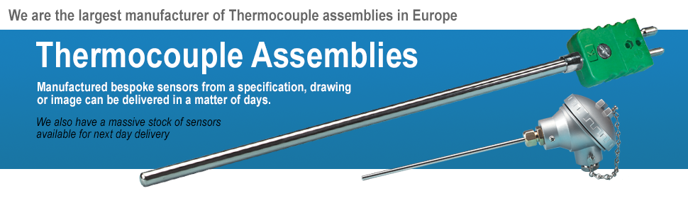
What is a Thermocouple? How do Thermocouples work?
Contents
- What is a Thermocouple?
- Understanding Thermocouple Functionality
- Cold Junction Compensation
- Material types for Thermocouples
What is a Thermocouple?
A thermocouple is a highly reliable temperature sensor used for measuring and controlling temperature in industrial, scientific, and commercial applications. The variety of available types and designs enable reliable measurements across a wide temperature range — from cryogenic conditions to high-temperature processes.
How Do Thermocouples Work?
A thermocouple consists of two different metal wires joined at one end to create a temperature-sensing junction (known as a 'hot junction'). When this junction experiences a temperature change, it generates a small electrical voltage (thermoelectric voltage), which corresponds to the temperature difference between the junction and the wire ends.
This effect, known as the Seebeck Effect, was first discovered by Thomas Johann Seebeck in the early 19th century. While any two dissimilar metals can generate a voltage, only specific thermocouple types (such as Type K, Type J, and Type T) provide stable, accurate, and predictable temperature readings across various environments.
Why Choose Thermocouples for Temperature Measurement?
Thermocouples are widely used in industries such as:
- Manufacturing and Process Control – Ensuring precise temperature regulation
- Automotive and Aerospace – Monitoring engine and exhaust temperatures
- Scientific and Healthcare Applications – Reliable, high-temperature measurements
Their durability, fast response time, and broad temperature range make them an ideal choice for demanding conditions.
Custom Thermocouples for Your Application
We specialise in custom-manufactured thermocouples designed for your specific application needs. Whether you require:
- Mineral insulated thermocouples
- Surface thermocouples
- High temperature ceramic sheathed thermocouples
Our expert engineers are here to help. Please contact us on 01895 252222 or use Live Chat for design advice.
Need advice on choosing a thermocouple?
Contact one of our experienced engineers on
01895 252222 or use the Live Chat button.
Popular Thermocouples
Mineral Insulated Thermocouples Rugged sensors, ideal for most applications. Vast choice of terminations e.g. pot seals, cables, connectors, heads etc.
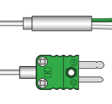
General Purpose Thermocouples
Rugged sensors, ideal for most applications. Vast choice of terminations e.g. pot seals, cables, connectors, heads etc.
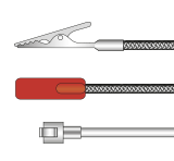
General Purpose Thermocouples
 A wide range of thermocouples to suit many applications. Hand held, surface, bayonet, bolt, patch styles etc.
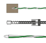
Thermocouples for Surface Measurements
A wide range of thermocouples to suit many applications. Hand held, surface, bayonet, bolt, patch styles etc.
Thermocouples for Surface Measurements
 A range of thermocouples to suit various surface temperature measurement applications.
Miniature Thermocouples
A range of thermocouples to suit various surface temperature measurement applications.
Miniature Thermocouples
 Ideal for precision temperature measurements where minimal displacement and a fast response is required.
Do I need a thermocouple or an RTD?
Please see our useful guide on whether to use a thermocouple or rtd for your application.
Understanding Thermocouple Functionality
A thermocouple is a simple yet highly effective temperature sensor that operates based on the Seebeck Effect. It consists of two different metal wires, joined at one end to form a measuring junction (hot junction), while the other ends are referred to as the cold junction.
When the hot junction is exposed to a temperature change, a temperature gradient forms between it and the cold junction, generating a small voltage (electromotive force, or EMF). This voltage, measured in millivolts, corresponds to the temperature difference along the conductor length.
To obtain an accurate temperature reading, a thermocouple display unit electronically references the cold junction to 0ºC and applies a formula to convert the millivolt signal into a temperature reading (°C or °F).
How Does a Thermocouple Generate Voltage?
A temperature gradient in an electrical conductor causes heat energy to move through it, creating an electron flow that generates an electromotive force (EMF). The size and direction of this EMF depend on:
- The temperature difference along the conductor
- The materials used in the conductor
This thermoelectric effect, discovered by T.J Seebeck in 1822, forms the basis of thermocouple operation.
However, in a single conductor, the sum of internal EMFs cancels out, meaning no measurable voltage is produced. This is why a thermocouple consists of two different metals each with distinct thermoelectric properties joined together. The difference in their EMFs creates a detectable output voltage, proportional to the temperature difference between the hot and cold junctions.
Temperature Gradients and Voltage Generation
The total EMF produced by a thermocouple also depends on the temperature distribution along the length of each conductor. As shown in Figure 2.1, different temperature profiles (a, b, c) can result in the same net EMF, provided each conductor is homogeneous and the end temperatures remain constant.
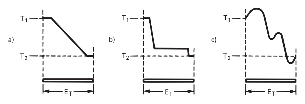
Figures 2.1 a,b,c: Temperature Distributions Resulting in Same Thermoelectric EMF
Where Is the EMF Actually Generated?
A common misconception is that the voltage is produced at the junction itself. In reality, the EMF is generated along the entire length of the conductor in the region where the temperature gradient exists.
The Role of the Measuring and Reference Junctions
A thermocouple does not measure absolute temperature—it measures the temperature difference between two junctions:
- Measuring Junction (M): Located in the medium where temperature is measured
- Reference Junction (R): Where the thermocouple wires connect to copper leads.
If the reference junction is held at a constant, known temperature, the temperature at the measuring junction can be accurately calculated from the thermocouple’s voltage output.
As illustrated in Figure 2.2, the voltage output (ET) remains the same for any temperature gradient distribution over the temperature difference T1 and T2, as long as the conductors exhibit uniform thermoelectric characteristics.
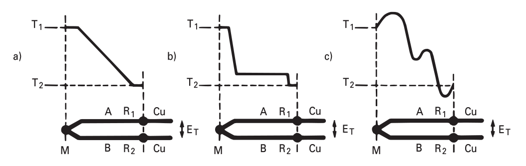
Figures 2.2 a,b,c: Thermocouple EMFs Generated by Temperature Gradients
Key Considerations for Accurate Temperature Measurement:
- Material Uniformity: Thermocouple conductors must be physically and chemically uniform throughout the temperature gradient. Any variations can introduce unwanted EMFs, leading to inaccurate readings
- Junction Placement: The reference junction must be maintained in a known and stable temperature (isothermal) environment. The measuring junction must be accurately positioned at the point where temperature is to be measured
- Extension Leads and Compensating Cables: These can be introduced into the thermocouple circuit to connect the probe to instrumentation. To avoid introducing unwanted EMFs, they must be made from compatible materials and kept at a uniform temperature along their length — or their junctions must be properly referenced and compensated.
- Extension wires are made of the same material as the thermocouple, while compensating cables use alternative materials that mimic thermoelectric behavior over a limited temperature range.
Final Takeaways:
- Thermocouples generate voltage only when a temperature gradient exists between the two junctions. Without a temperature difference, no voltage is produced
- Accuracy depends on uniform thermoelectric properties of the conductors
- A functional thermocouple circuit must contain two different metals in a temperature gradient

Cold Junction Compensation
Thermocouple calibration tables relate output voltage to the measuring junction temperature, assuming the reference junction is held at 0°C. If the reference temperature varies, the voltage output changes, leading to inaccurate readings. To ensure precise measurements, cold junction compensation is required.
Historically, this was achieved by immersing the reference junction in melting ice, maintaining a stable 0°C. Figure 5.1 illustrates a Dewar flask setup, a simple yet highly accurate method still used in laboratories today. However, this approach is impractical for industrial applications due to regular maintenance needs and potential errors (e.g., ice melting and floating on water at 4°C).
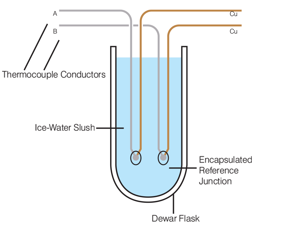
Figures 5.1: Dewar flask with Reference Junctions
Modern Cold Junction Compensation Methods
Industrial thermocouples use automated systems to maintain a stable reference temperature:
-
Temperature Controlled Enclosures:
- Reference junctions are placed inside a Peltier-cooled enclosure, holding them at 0°C with minimal error (±0.1°C)
- This method offers excellent accuracy and stability, aligning with standard thermocouple reference tables
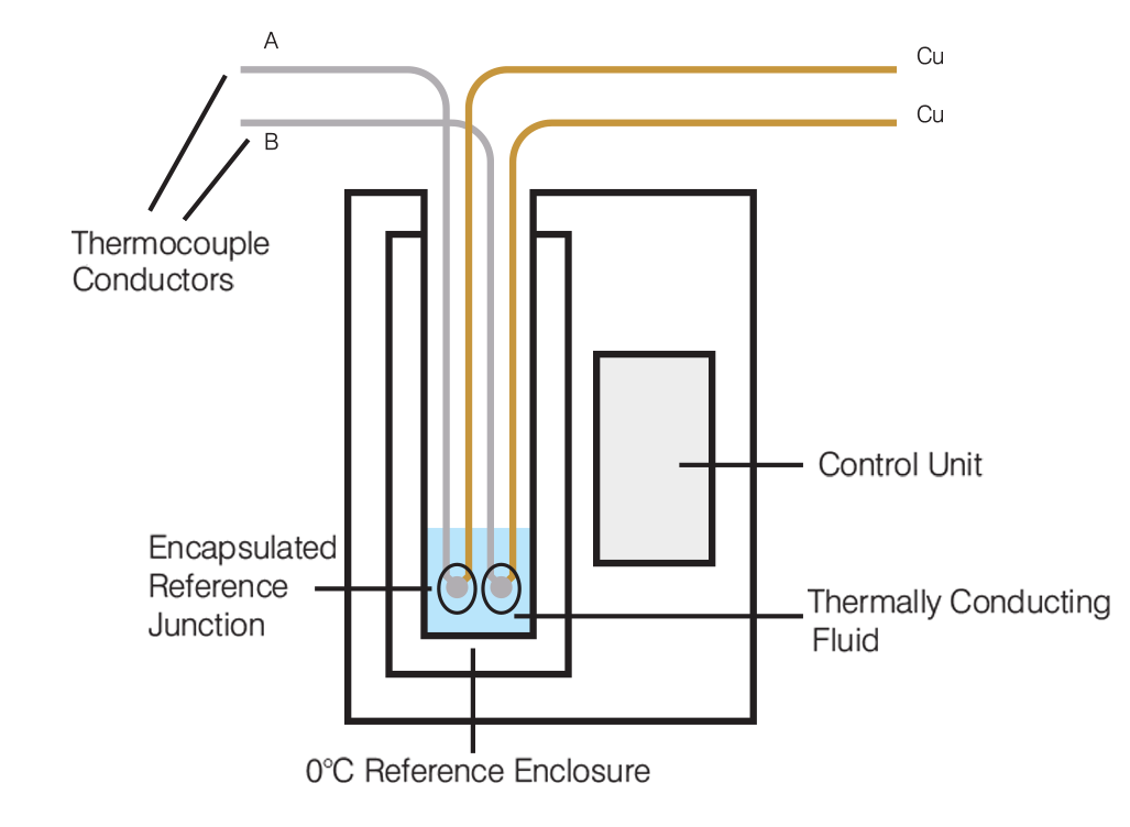
Figures 5.2: Temperature controlled enclosure
-
Electronic Cold Junction Compensation:
- A temperature sensor (e.g., thermistor, RTD, or transistor) near the reference junction measures its temperature
- A correction voltage is then added to the thermocouple signal, either electrically or via software calculations in instruments like data loggers, temperature controllers, and digital thermometers
- Many modern instruments automatically apply cold junction compensation, eliminating the need for an external reference
-
Multi-Thermocouple Systems:
- Large installations use racking systems with 100+ reference junctions inside a temperature-controlled enclosure or a thermally stable metal block
- The block’s temperature is monitored, and compensation is applied electronically or numerically for each thermocouple
-
High-Temperature Reference Units:
- For environments with high ambient temperatures, specialized enclosures maintain a known reference temperature
- The thermocouple readings are adjusted to the equivalent 0°C values using standard correction factors
As long as the reference temperature is known, the measuring junction temperature can be calculated with precision.
See our dedicated thermocouple Cold Junction Compensation page
Material Types for Thermocouples
Most conducting materials can generate a thermoelectric output, but practical thermocouples require:
- A wide and stable temperature range
- Strong signal output
- Good linearity and repeatability
After decades of research by suppliers, calibration labs, and academia, thermocouple materials now cover temperatures from -270°C to 2,600°C.
Standard Thermocouple Types
Thermocouples are categorized into two main groups:
-
Rare Metal Types (Platinum-based, e.g., Type S, R, B)
- Most stable but expensive
- Used up to 2,000°C (short-term: 3,000°C)
- Lower signal output than base metals
-
Base Metal Types (Nickel and Iron-based, e.g., Type K, Type J, Type T)
- More affordable, commonly used in industry
- Typical range: 0 to 1,200°C (wider for short-term exposure)
- Higher signal output than rare metals
Key Considerations
- Type K instability: Known for drift over time and temperature cycles
- Type N (Nicrosil/Nisil): Designed to improve stability, offering base metal pricing with rare metal performance
- Standardisation: Governed by BS EN 60584-1 (formerly BS 4937) and IEC 60584, using letter designations